- Demand Relation...
- Demand
- Price and demand
- Demand and tota...
- Changes in demand
The Demand Relationship
Economics is very much concerned with the operation of markets as co-ordinators of exchange. The most common co-ordinators are markets and organisations. In the case of markets, the price mechanism ensures only one equilibrium position is reached where consumers’ demand meets producers’ supply. The outcome is efficient as consumers buy the quantity of the good or service they demand and producers sell the quantity they supply at the market equilibrium price. There are no shortages or surpluses. The price includes all the necessary information for producers and consumers.
While the focus in economics has historically been on the study of markets as exchange mechanisms, new perspectives to the topic of co-ordination were introduced by Coase (1937) who posed the question as to why so much economic activity took place within hierarchies if markets were so efficient. This resulted in a theory contending that the use of markets comes at a cost, which Coase coined transaction cost. This subject was further developed by Williamson who outlined the sources of transaction costs and set out governance modes to co-ordinate exchange.
Well-established transaction cost economics is used to explain many of the current phenomena in the business world. Thus, for example, it provides insights into the reasons why a large number of firms have decided to outsource or transact with other firms externally as developments in telecommunications and I.T. have reduced transaction costs. Our focus in this unit, nevertheless, will be on the microeconomic study of markets. Co-ordination exchange within hierarchies and transaction cost economics will be explored in Study Guide 1 and in the course of the workshop.
Demand
The term demand refers to the willingness and the ability of consumers to consume. The concept is crucial in economics as it concerns how and why consumers make decisions. This section analyses the reasons and factors explaining these consumption decisions and the relationships existing between demand and its explanatory constituents.
The difference between the terms ‘quantity demanded’ and ‘demand’ is of utmost importance in analysing consumer theory. While the former refers to the amount of a good or a service consumers are willing and able to buy, demand refers to the whole relationship existing between the quantity demanded and the factors that determine this quantity, such as price, utility or price of a substitute. The quantity demanded of computers in a country, for example, refers to the amount of computers consumers in the country are willing and able to buy at a given price. The demand for computers, on the other hand, refers to the relationship existing between the quantity demanded and its determinants such as the price, income or the price of a substitute product. The demand is therefore seen as a function linking the quantity demanded to its determinants.
Thus, the quantity demanded of Dell desktop computers, for example, could be explained by their price, the income of consumers, the number of potential consumers, the price of substitute goods such as laptop computers or HP computers, the future expected price, etc.
Price and demand
The price of a good is commonly seen as the most important determinant of the demand. Usually, there is a negative relationship between the price and the quantity demanded of a good. This statement is known as the Law of Demand and illustrates the fact that consumers tend to buy more of a good as its price goes down and buy less as its price increases. Nevertheless, while constituting exceptions, it is worth mentioning some instances when consumers react positively to price increases. One such example refers to ‘snob’ goods such as luxuries which are consumed because of their status symbols. Our focus, will be on the more general case where there is a negative relationship between the price and the quantity demanded.
The demand schedule is a table summarising the prices and resulting quantities demanded of a product. Table 1 shows an example of a demand schedule for computers in a country:
| Price (in $) | Quantity demanded (in millions) |
| 800 | 10 |
| 850 | 9 |
| 900 | 8 |
| 950 | 7 |
| 1000 | 6 |
The graphical representation of the demand schedule is known as the demand curve and is illustrated in Figure 1.
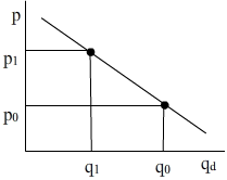
The demand curve (D) illustrates the negative relationship between price (p) and quantity demanded (qd) through a negatively sloped function. Our depiction of a linear demand function is due to simplicity. It is a useful assumption as it is enough, for the purposes of our analysis, to highlight the Law of Demand through a negative relationship between the quantity demanded and the price. The demand function for most goods and services in the real world, nevertheless, is more likely to be a curve.
Price changes result in movements on the demand curve and in turn, changes in the quantity demanded. Figure 1 illustrates that an increase in the price of a good from p0 to p1 results in a reduction in the quantity demanded of the good from q0 to q1, ceteris paribus. In contrast, a reduction in the price would result in an increase in the quantity demanded. This situation could be illustrated by the increase in the quantity demanded of computers since the 1980s which resulted from their reduction in price.
Changes in prices result in changes in the quantity demanded. In contrast, changes in the determinants of the demand for goods or services, other than price, result in changes in demand. These are illustrated as shifts of the demand curve.
Demand and total revenue
The demand function constitutes the main building block in the study of the consumer in the economy. Its use is key in determining the ability of a firm to generate revenue from the sale of goods or services and in assessing profitability when contrasted to the costs incurred in producing these goods. Our focus within Kaelo is to illustrate the relationship between the demand and the total revenue functions.
Revenue is the amount of money generated from the sale of goods or the provision of services. Thus, if p is the price charged per unit of output sold and q is the amount of output, the total revenue is the multiplication of p times q:
A quick look at the total revenue function reveals how closely linked this function is to the demand function illustrated:.
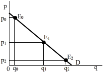
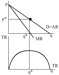
Thus, in Figure 2 the total revenue generated when the organisation charges p0 and sells q0 is measured geometrically by the area delimited by rectangle E0q00p0. A reduction in the price of the good from p0 to p1 results, through the negative relationship between price and quantity, in an increase in the quantity demanded from q0 to q1 and in turn, in an increase in the total revenue generated to area E1q10p1. Nevertheless, further reduction in the price to p2, result in an increase in the quantity demanded to q2 which reduces the total revenue to the area delimited by E2q20p2. This suggests that total revenue increases while output increases up to a point (q*), after which, further increases in output result in reductions in total revenue. The relationship between the demand curve (D) and the total revenue function (TR) is illustrated in Figure 3.
This relationship (key to understanding the Baumol model) will be explored in more detail in Managerial Economics as it provides insights into the optimal revenue maximising price. Suffice to mention that close scrutiny of the demand function will permit organisations price at a level which maximises revenue. This, in turn, can increase market share when it is assumed competitors do not react to price reductions or increases.
Further observation of Figure 3 reveals the illustration of the average revenue function (AR), which coincides with the demand curve, and the marginal revenue (MR) function. Their importance resides in their contribution to decision making using marginal analysis and to the evaluation of profitability through the superimposition of cost functions on demand and revenue diagrams. In this context, the average revenue is defined as the revenue generated in selling, on average, one unit of output. The average revenue function is summarised below,
Because the average revenue, due to its definition, is calculated as total revenue divided by output, its value will be the price, which is determined by the demand function. Thus, the average revenue and the demand functions coincide as demonstrated by the expression above.
Furthermore, the marginal revenue is defined as the extra revenue received when selling one extra unit of output. Because the price decreases as the business sells extra units of output, the extra revenue received will also decrease. Therefore, the negative slope of the demand relationship in turn determines the negative slope of the marginal revenue function. Study Guide 1 in Managerial Economics uses the crucial marginal revenue function coupled with the marginal cost function to locate the profit optimising output.
Changes in demand
This section returns to the analysis of the factors determining demand. Changes in any of the factors determining demand other than price result in shifts of the demand curve. These are in contrast to movements along the demand curve which result from changes in the price of the good or service. An increase in demand will thus result in a shift of the demand curve outwards to the right and a reduction in demand will result in a shift of the demand curve inwards to the left. While different variables determine the demand for each good, we will focus on those common to most products.
- Income
The effects of changes in income on demand are very important not only because they determine the type of good under study, but also because they offer information to businesses on the likely movement of demand through the business cycle. Two different types of goods can be distinguished depending on whether a change in income, ceteris paribus, has positive or negative effects on demand. These are known as normal and inferior goods respectively.
Normal goods are those summarising a positive relationship between income and demand. Thus, an increase (decrease) in income results in an increase (decrease) in the demand for a normal good, ceteris paribus. Examples of normal goods include clothes, electronic goods or cars. Increases in income for normal goods in turn translate into shifts of the demand curve to the right as illustrated by Figure 4(a), while reductions in income result in shifts to the left as illustrated by Figure 4 (b).
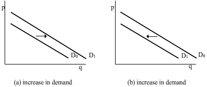
Inferior goods, on the other hand, are those summarising a negative relationship between income and demand. Thus, an increase (decrease) in income results in a decrease (increase) in demand for an inferior good, ceteris paribus. Examples of inferior goods include low quality food. Increases in income for inferior goods translate into shifts of the demand curve to the left as illustrated by Figure 4(b), while reductions in income result in shifts to the right as illustrated by Figure 4(a).
- Price of related goods
Some goods are related in such a way that a change in the price of one good results in a change in the demand for other goods. Relations between these goods can be of substitutability or complementarity. When the increase (decrease) in the price of one good results in an increase (decrease) in the demand for the other good, ceteris paribus, the two goods are substitutes. An increase in the price of computers, for example, is likely to result in an increased demand for laptops to the degree that the two goods are substitutes. Thus an increase (decrease) in the price of one product A results in an increase (decrease) of the demand for a substitute product B which is, in turn illustrated by a shifting demand curve for product B to the right (left).
When the increase (decrease) in the price of one good results in a decrease (increase) in the demand for the other good, ceteris paribus, the two goods are complements. An increase, for example, in the price of computers is likely not only to decrease the demand for computers but for printers, as well. Thus an increase (decrease) in the price of one product A results in a decrease (increase) in the demand for a substitute product B which is in turn illustrated by a shifting demand curve for product B to the left (right).
- Population size
The greater the population size, the greater the demand for a product, ceteris paribus. An increase in the population size shifts the demand curve to the right as illustrated by Figure 4(a). In contrast, a decrease in the population size results in a shift of the demand curve to the left as illustrated by Figure 4(b).
Computer companies, for example, expand their operations to new countries in order to increase the demand for their products. This may be one of the reasons for Lenovo’s acquisition of IBM personal computers’ division in 2005 which permitted Lenovo the use of IBM’s existing capacity in a large number of countries to extend its operations and introduce itself into the PC markets in the West. Other explanations for organisational growth into new markets are valid as well. In this context, organisations may decide to expand their operations into new countries in order to minimise the risk of exposure to the contingencies of a particular economy or to reduce production costs. The reasons determining the boundaries of the organisation will be studied in the Managerial Economics Study Guides.
- Future expected prices
A further factor to consider is the future expected price. Thus, for example, a potential investor’s decision to purchase stock in the exchange market is influenced by her perception of the evolution of future prices. If she expects prices to go down she might delay her purchase or reduce her current demand. If she, in contrast, expects prices to go up in the future, she is more likely to purchase now.
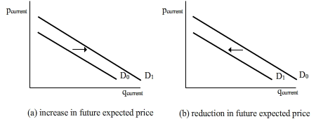
Therefore the role of expectations as illustrated by Figure 5 is very important in economics as it influences current and future demand. Similarly, future prices influence producers’ current and future supply decisions.