- Indiffe...
- Utility
- Indiffe...
- Convex S...
- Characte...
- The budg...
- The indif...
- Applicati...
- Exercises
Indifference Relationship
he concept of indifference is a key driver of the management models. It helps to identify a trade-off between any two financial variables (for example, profits and market share) provided a third variable remains unchanged. In economics, utility is used to measure the well-being obtained by consumers from the consumption of output. The measurement of utility, in turn permits us to summarise the preferences of the consumer. Furthermore, the consumer’s income and the prices of goods are used to estimate consumption possibilities.
Many CEOs do not reveal the third variable, and the guessing game is captured later in our discussion on Signalling. In the interim, proceed as follows to get a flavour of the indifference relationship as applied to management:
- Step 1: What could the 3rd variable be? Value (Marris), Revenues (Baumol), Costs, Growth?
- Step 2: Click on sub-menu The Indifference Equilibrium
- Step 3: Click on sub-menu Applications
- Step 4: Click on sub-menu Exercises
Utility
Utility is defined as a measure of the satisfaction or well-being consumers obtain from the consumption of goods and services. Thus, if a consumer drinks 3 cups of coffee, her utility would be measured by the satisfaction she would gain from the 3 cups.
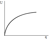
The relationship between the quantity of a good or a service consumed (q) and the utility obtained (U) is summarised by a positively sloped utility function. The utility function is expressed below:
The term marginal utility, on the other hand, measures the change in utility resulting from a one unit increase in the consumption of a good or service. It refers to the contribution to utility resulting from consuming one extra unit of a product. The contribution to utility from consuming the third cup of coffee would therefore be the marginal utility of the third cup.
While we will assume, for simplicity that the higher quantity of a good or service consumed, the higher the total utility, which determines the positive slope of the utility function, we will also assume that extra units contribute less to total utility or diminishing marginal utility.
This assumption results from the contention that consumers tend to grow tired of goods and services as their consumption increases, and it is known as the ‘Law of diminishing marginal utility’. Figure 1 illustrates the representation of a positively sloped utility function, where utility increases with quantity consumed, and where marginal utility (the slope of curve in Figure 1) diminishes with higher output.
One of the main problems of the concept of utility resides in its difficulty to be measured. Consumers cannot put a quantitative value to the utility they obtain from consumption but only order. Thus, consumers are able to qualitatively put an order to their preferences and state that they prefer one consumption bundle to another but not by how much. Notwithstanding this limitation, the use of utility functions continues to constitute the foundation of the theoretical study of consumer behaviour analyses. The concept of utility is used in a number of applications in Managerial Economics. For example, in decision making analysis utility functions are used to measure decision makers’ attitude to risk.
Indifference curves
The analysis of utility could be extended to measure the well being obtained from the consumption from bundles of two or more goods. This permits economists to analyse of a trade-off between two goods. In this sense, one must define indifference curves as curves which summarise the bundles of two goods that yield a constant level of utility. Consumers are thus indifferent to any of the bundles of goods along an indifference curve since utility is constant. Figure 2 illustrates an example of an indifference curve:
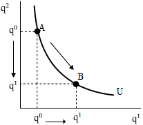
The level of utility is held constant along the indifference curve. Thus, consumers are indifferent between bundle A or B in Figure 2 as they are on the indifference curve where utility is held unchanged. As consumers move from bundle A to bundle B, they give up in the consumption of q2 in order to increase in the consumption of good q1 holding utility constant. Consequently, there is a trade off between the consumption of the two goods.
While an indifference curve allows comparisons between bundles which yield constant utility, one must illustrate an indifference map if it is wished to analyse bundles with different utilities. There is an indifference curve for every level of utility. But because there are infinite levels of utility, there will be infinite indifference curves. An indifference map plots a whole set of indifference curves.
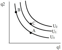
Higher levels of utility are depicted in Figure 3 as higher indifference curves. Thus, consumers are indifferent between bundles A and B located on the same indifference curve but prefer bundle C to bundles A and B as it is on indifference curve U1 connected to a higher level of utility. In turn, consumers prefer any bundle on U2 to bundles on U1.
Convex Slope of indifference curve
One key feature of the indifference curves analysed up to this point is that they are convex to the origin. This implies that their slope changes. As one moves on the indifference curve downwards, the slope decreases. The reason for the diminishing slope will be explained later.
The slope of the indifference curve is known as the ‘marginal rate of substitution’ (MRS) and it measures the amount of one good that must be given up in consumption in order to increase the consumption of the other good by one unit holding utility constant. In other words, it measures the opportunity cost of consuming one extra unit of a good. Mathematically, the MRS at one point on the indifference curve is measured by the derivative of the utility function with respect to the quantity demanded of one good at the particular point and is illustrated as the slope of the tangent line to the utility function at the point.
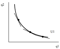
Figure 4 illustrates the ‘Law of diminishing MRS’. As a consumer decides to increase her consumption of the good or service measured on the horizontal axis, she is willing to give up less of the good measured on the vertical axis. The MRS thus diminishes.
Characteristics of indifference curves
There are three main characteristics of indifference curves we will use for the purposes of the Managerial Economics course. Note: that indifference curves could differ from the ones presented here. Their shape is not necessarily convex to the origin and in some cases they are not negatively sloped, however, the most general analysis of indifference curve contains the following characteristics:
- Negatively sloped: Why?
The negative slope of the indifference curve illustrates the fact that in order to consume higher amounts of one good consumers must give up in the consumption of the other if they are to hold utility constant. The slope of the indifference curve, thus, determines a trade-off.
- Convex to the origin: Why?
As noted above the ‘law of diminishing MRS’ results in a convex indifference curve: but why does this observation or ‘law’ obtain? The ‘Law of diminishing marginal utility’ is the key to understanding the ‘Law of diminishing MRS’.
As consumers consume more of a good or service, it was contended they would obtain smaller marginal utility. This means consumers value a product less as they consume additional units. Thus, given the trade-off decisions between two goods, consumers will value a good less the more they consume which means they will be willing to give up less of the other good. Hence the rate of substitution between the two goods (MRS) is declining.
- Indifference curves do not intersect: Why?
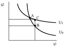
Because A and B in Figure 5 are bundles on the same indifference curve U0, they are equally preferred. Likewise, because A and C are in turn bundles on the same indifferent curve U1, they are equally preferred. Because consumers are indifferent between A and B and A and C, we can conclude they are indifferent between B and C. However, a closer look to Figure 5 shows that, while including the same amount of q1, bundle C includes a higher amount of q2 than bundle B, which means consumers would prefer C to B. This contradicts the previous contention that consumers were indifferent between bundles B and C. Therefore utility curves cannot intersect.
The budget constraint
The budget constraint summarises the bundles of two goods a consumer can afford given her income and the prices of the goods. Indifference curves summarise the subjective preferences of consumers, but do not illustrate their ability to consume them. Thus, the superimposition of the budget constraint on the indifference curve map is necessary if one wishes to analyse the highest utility one consumer could obtain given her budget.
The budget constraint can be expressed in terms of the income of the consumer (M), the price of and the price of :
where p1q1 represents the expenditure on q1 and p2q2 represents the expenditure on q2.
Figure 6 illustrates the budget constraint:
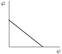
Bundles of goods included in the region below the budget constraint illustrated in Figure 6 can be afforded by consumers who do not spend all their income. The bundles on the budget constraint can be afforded when consumers spend all their income. Bundles included in the region above the budget constraint cannot be afforded even when consumers spend all their income.
Other key points in the analysis of the budget constraint concern its slope and position. The slope of the budget constraint is determined by the relative prices of the two goods with a negative sign to indicate the negative slope: . An increase in p1 relative to p2 results in a steeper budget constraint. On the other hand, a reduction in p1 relative to p2 results in a flatter budget constraint. The budget constrain will shift upwards to the right when consumers’ income increases and will shift downwards to the left when income decreases.
The indifference equilibrium (point of tangency)
The Consumer’s objective is to optimise utility subject to a budget constraint. Thus, consumers try to reach the highest indifference curve given their income and the prices of the goods.
The highest indifference curve that can be reached is the one that shares a tangency point with the budget constraint.
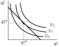
Figure 7 illustrates that the highest indifference curve consumers can reach is U1 as it shares a tangency point with the budget constraint. Consumers optimise their utility when they consume q1* and q2*. At this equilibrium point, the slope of the budget constraint is equal to the MRS.
Applications of the theory to management models
Our interest in the analysis of indifference curves and budget constraints is rooted in their role in explaining management decisions and in the description of the objective of businesses under the separation of ownership from control. These issues will be explored in Study Guide 1 in the Managerial Economics course where it is contended that indifference curves can be ascribed to management behaviour. In this context, managers may derive utility from both making profits and revenue, but there may be a trade off between the two of them which can be illustrated with the use of an indifference curve. In their pursuit to maximise utility, nevertheless, managers are constrained by a profit function where output acts as a proxy for sales.
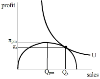
Figure 8, in this context illustrates Baumol’s contention that due to the separation of ownership from control in modern corporations, management who have discretion over the resources of the firm, may be able to increase revenue above the level consistent with profit maximisation as long as their revenue contributes to their utility. The tangency point between the profit constraint and management’s indifferent curves occurs to the right of the profit maximising level of revenue.
Study Guide 1 contends that the use of indifference curves to ascribe management behaviour can also be used to illustrate other theories built in the context of the agency relationships resulting from the separation of ownership from control such as Marris’ theory of growth and Williamson theory on management discretion. These issues will be explored in detail in Unit 1 and in the workshops in the Managerial Economics course.
Realism of a Managerial Indifference Curve
Finally, how realisic is the concept of a managerial indifference curve? Ask yourself the following question: does a manager have a particular preference as to where he/she may be transfered in the modern corporation? Why do management have perks, spacious offices, and valet car parking? Are management concerned about the quality of the product produced at the plant, about industrial relations at the plant, about salaries, about possible takeover bids or merger possibilities? If the answer is in the affirmative, then modern management can be ascribed a utility function with an underlying convex indifference curve.
The concept of a managerial indifference curve is not too unrealistic. Again ask yourself: does management allow the quality of life, working conditions, employee satisfaction, good industrial relations to impact on how he/she performs the duty and task of management. If the answer is in the affirmative then management has a utility function - rather we can ascribe a utility function to management. In other words, there are numerous other non-quantifiable intangible events which impact on both the management and the production decision-making process. We address the latter in Unit 2.
The desire for perks and equity stakes across top management and the search for non-proft compensation in a job, translate easily into the arguments of a utility function. Hence, the more risk-averse management is, the more the shape of the proposed utility function is concave; in other words, managers are fundamentally risk-averse in the complex environment of a modern firm, an environment which is overshadowed by many constraints and stakeholder interests. How management ‘manage’ the risks involved will be looked at in the Workshops.
Exercises
Exercise 1
Examine the interrelationship between the Marris model and the Williamson model with respect to divergence from the profit maximizing level. As discussed earlier, these two models employ a manager utility function represented by U. The Marris utility function has two arguments:
The Williamson utility function likewise has two arguments:
Figure 3 in the Study Guide superimposed the Williamson utility curve on the discretionary profits function. Contained within Figure 5(c) in the Study Guide is Marris’ balanced growth curve, represented by [abcd] and imported into Figure 9 of this Workbook as the concave curve .
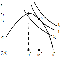
Notice the similarity between Figure 5(c) in the Study Guide and Figure 9 here, particularly when we superimpose the Marris utility function on the balanced growth curve as in Figure 9. An optimal point is reached, point A in Figure 9, between the objective function [either the discretionary profits or the balanced growth curve] and the utility function. Point A forces the firm to diverge from the profit maximizing level. This is one of the more important results of the managerial models in general and of the Marris model in particular. The location of point A indicates that, contrary to the traditional assumptions in finance and economics, the managerial firm will not maximize value per share. Instead the firm will increase growth at the expense of profit and of valuation until it attains its optimum level of managerial utility.
Exercise 2
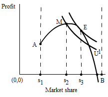
Is it always the case that in a multi-goal firm that one goal has to be abandoned in favour of another? In attempting to answer this question we would like to advance an idea for future research into the theory of firm behaviour and the objectives of economic organizations. It is an issue to which we shall return in the workshops. Taking a lead from Shubik’s [1961] model, wherein he analysed the behaviour of a two-goal firm, we generalise and state that firms have a two-goal objective. In the illustration in Figure 10, we consider profit and market share as two possible goals which would enter into the manager’s utility function. The constraint that is imposed by shareholders and external financiers manifests itself in a minimum market share, s1 in Figure 10.
Exercise 3
Explain the concavity of the trade-off diagram, Figure 10? The concavity of the trade-off diagram can be explained as follows:
1. the firm is not a monopolist and does not dominate the market,hence the upper limit, B, on market share is less than 100%,
2. the firm must attain a minimum market share, s1, before returning a positive [supernormal] profit. A maximum market share exists at s2 and one could define a satisficing market share as falling between s1 and s2.
At point M in Figure 10, the maximum market share is attained with a manager utility level represented by utility curve U1. The manager could attain a higher level of utility if a higher market share is acquired, but at a cost of reduced profits. However, at M, the subjective marginal rate of substitution [MRS] between profits and market share exceeds the objective [market determined] marginal rate of substitution. This suggests that the firm, in its own interests, should sacrifice profit for market share in order to equate the MRS’s at the equilibrium point E. The essence of this approach is that multiple goals call for compromises, not the complete abandonment of one goal for another.
Exercise 4
Comment on the sequential moves undertaken by the firm, in particular from πA to πE and from πM to πE. The firm has moved sequentially from s1 to s2 and from the profit levels πA to πE. The move from πA to πE is favourable and may be interpreted as a long term strategy. The move from πM to πE, however, is unfavourable with respect to profits as it involves a reduction in profits. This move could represent a short run objective where short run profits are sacrificed for an increase in market share. Collectively over the time horizon, the firm has moved from an initial point A to a final point E. The choice of initial starting point will predetermine whether the move is beneficial to the firm.