Elasticity and Total Revenue [TR] Test

The change in total revenue, denoted by ΔTR, can be conveniently expressed as:

The ratio ΔTR/Δq is the marginal revenue accruing to the firm. As defined it is the slope of the total revenue curve. The TR test is harnessed by the changes in quantity Δq which can either be elastic when Δq > Δp or inelastic when Δq < Δp. There is the possibility of an equi-proportionate change so that Δq = Δp. The crucial term in deciding the direction of ΔTR is inevitably the Δq term. In other words, a management decision to increase price [identified a later chapter as the strategy of premium pricing] is contingent on the price range being inelastic so that Δq < Δp;conversely the decision to reduce price [identified as the strategy of down-sizing on price] is contingent on the price range being elastic so that Δq > Δp. Hence, increase price in the inelastic price range and decrease price in the elastic price range.

However, along the demand relationship as illustrated in Figure 1(a), there are trigger price points e,f,g,h, where the price range changes from elastic to inelastic or from inelastic to elastic. As a guide for management, on average the price ranges are more elastic in the higher price ranges such as [ef] where p > q and more inelastic in the lower price ranges such as [gh] where p < q on a demand function. For example, a strategy of down-sizing on price could backfire, particularly if the reduced level of price transcends the trigger price into an inelastic price range, where a reduced price generates a loss in revenue. We refer to this as the Marlboro© effect.

The total revenue test

One of the main applications of the concept of the price elasticity of demand to managerial decision-making concerns the relation existing between the values of elasticity along a demand function and the total revenue function. Note the value of the point price elasticity of demand changes along a linear demand function. Management can then implement appropriate price strategies in order to increase total revenue as long as they know the elasticity of the demand faced by the business.

One useful starting point is the analysis of the formula used to calculate the point price elasticity of demand. This formula is composed of two main parts: the derivative of the demand function with respect to price (dqd/dp) and the price to quantity ratio (p/qd). Because the geometric interpretation of the derivative of a function at one point is the slope of the function at that point, the derivative of the demand function must be constant along the linear demand function. In contrast, the second term in the formula concerns the ratio price to quantity demanded which decreases as one moves downwards along the demand function.

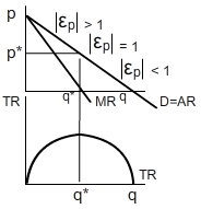
The value of the price elasticity of demand thus decreases as the price is reduced and the quantity demanded increases. This issue is crucial in economics as it implies that a linear demand function is always split into different price elasticity ranges: an elastic range for high prices, a point where the demand is unit elastic and an inelastic range on the bottom of the demand function. The elastic and the inelastic ranges of the demand function coincide with the sections of the total revenue function that increase and decrease respectively as the quantity demanded increases.

The level of output where the demand is unit elastic in turn coincides with the revenue optimising level of output. Figure 2 extends the illustration of the relationship between the demand and revenue functions to include the elasticities consistent with different sections of the demand function. This relationship is known as ‘the total revenue test’.

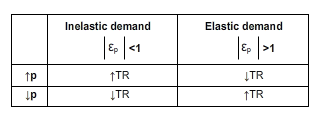
The relationships summarised by Figure 1 offer prescriptions for management optimising revenue. Thus managers should reduce prices when the demand is elastic and increase prices when the demand is inelastic. Table 1 summarises the effects of increases and decreases in prices on total revenue

The usefulness of the total revenue test resides in the prescriptions it offers to revenue optimising managers. Nonetheless, the test can be criticised since it does not consider the competitive response of rivals in oligopolistic industries. While consumers increase the demand for a good when a firm decreases its price on the elastic range of the demand curve in order to increase revenue, competitors may match a price decrease so as not to lose market share. Other problems connected to the test are discussed in much detail in Study Guide 3 in the Managerial Economics course.

Determinants of price elasticity of demand

The price elasticity of demand varies from one product to another. The demand for some products like petrol is very inelastic, while the demand for other products such as luxuries is very elastic. This section outlines some of the determinants of the price elasticity of demand.

• The number and closeness of substitute products. This is one of the most important determinants of the price elasticity of demand. The possibility of buying substitute products implies customers’ response to price changes is huge compared to situations where there are no substitutes. In this sense, the smaller the number and the more differentiated products are, the more inelastic the demand function. In contrast, the higher the number and the closer substitute products are, the more elastic the demand. Thus, customers decrease the demand for green beans more than proportionately when their price is increased since there are many other vegetables they can buy but keep buying petrol even when its price increases as they cannot use other substitutes. The demand for vegetables is therefore quite elastic while the demand for petrol is quite inelastic. Producers could try to differentiate their products from those produced by their competitors in order to gain sustainable competitive advantage which can, in turn, result in more inelastic demands and the possibility, through the total revenue test, to increase prices and profits.

• The time period. The longer the time period under consideration the more elastic the demand is likely to be. This is due to the fact that consumers are able to adapt to price changes over time. Thus, for example, while the demand for petrol is very inelastic in the short run, it tends to be more elastic over time as consumers find other substitutes. A consumer who uses the car to get to work every day will still have to buy petrol even if its price doubles in the short run, however, in the long run, she may decide to use public transport, buy a smaller car or even change the job. Europe became more efficient over time in the use of petrol after the 1970s petrol crises by using less energy, promoting smaller engines than their American counterparts and by encouraging the use of other energy sources like gas.

• Proportion of income spent on the good. The lower the proportion of income spent on the good, the more inelastic the demand is likely to be. In contrast, the higher the percentage of income spent on the good, the more elastic the demand is likely to be. If a consumer with a yearly income of £39,000, for instance, buys 5p worth of chewing gum every morning, she is not likely to stop buying chewing gum when its price goes up by 100 per cent to 10p because 10p represents a minute percentage of total income. In contrast, a miniscule percentage change in the price of a car, which constitutes a high percentage of her yearly income, would have a large effect on the consumer’s decision to buy it.

• Habit creating and addictive goods. When consumers are addicted to some products, they are not likely to reduce their consumption much when their price increases. Thus, goods such as cigarettes, alcohol or drugs are consumed even when their prices increase. Their demand is inelastic. Governments who need a quick source of income tend to increase indirect taxes in these goods because due to their inelastic demand, consumers will buy them even when their prices increase.

• Luxuries and necessities. The demand for luxuries tends to be more elastic than the demand for necessities. Consumers could stop buying luxuries should their prie increase but must buy necessities even when their price is increased.

The cross price elasticity of demand

In some cases goods are related to each other in such a way that changes in the price of one good results in changes in the quantity demanded of another good. In this sense, when goods are related, they can be complements or substitutes. The ‘cross price elasticity of demand’ indicates whether or not any goods are related and measures the strength of the relationship.

The cross price elasticity of demand measures the response of the quantity demanded of one good B to changes in the price of good A. the formula that measures the cross price elasticity of demand is expressed below.

where εAB is the cross price elasticity of demand, %ΔqB is the percentage change in the quantity demanded of product B, and %ΔpA is the percentage change in the price of good A.

When an increase (reduction) in the price of good A results in a reduction (increase) in the quantity demanded of good B, the value of the cross price elasticity of demand is subsequently negative. The goods are complements. Computers and printers represent an example of complement goods.

In contrast, when an increase (reduction) in the price of good A results in an increase (reduction) in the quantity demanded of good B, the value of the cross price elasticity of demand is subsequently positive. The goods are substitutes. Examples of complement goods include coffee and tea (although in some cultures they are taken together).

The closer the cross elasticity of demand is to 0, the less related two products are. The more negative and the more positive the cross price elasticity of demand, the stronger complements and substitutes the pair of goods are respectively.

Table 3 summarises the relationships depending on the cross price elasticity of demand.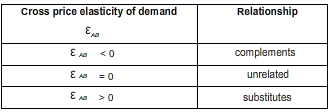

The cross elasticity of demand is useful in determining which are the products competing in the same industry. It is crucial for example to know any firms’ substitute products in the analysis of the likely response of competitors to the implementation of any strategy.

The cross price elasticity is also used in the study of a relevant market as a first step in antitrust investigations. Thus, for example, should a firm report a competitor for anticompetitive practices such as predatory pricing or abuse of dominant position to the competition authorities, it will firstly need to prove that they compete in the same market. The cross price elasticity of demand is used to determine whether or not the goods produced by the two firms are substitutes.

The Strategic TR Test

In this section we focus attention on price strategies which have a few elements of direct interest to management. There is the tangible relationship between price - denoted by the price vector P in order to highlight the different product prices - and total revenue via the TR Test and between price, total revenue and profits:

The calculation of prices depends on the price elasticity of demand εp, but strategic prices depend on the

• price hierarchy,
• rival reaction, and
• product type.

In other words if the rival price is lower down on the hierarchy than the anticipated price reduction by the representative firm, there is no retaliation by the rival.. If the product pair are net substitutes any change in price should have no adverse effects on the quantity of the rival substitute produced. This further reinforces the absence of the need for retaliation as the price reduction does not obtrusively encroach on rival market shares.

This gives us a second link between the price vector P and a vector P' = {p1',p2',...pm'} of rival hierarchical prices, as follows:

The ratio Λ = will determine how TR responds to a Δp. If Λ > 0 the price change is tolerated by rival firms and if Λ < 0 there will be retaliation, so Δp may not realise the TR objectives. If there is a product portfolio for the stakeholder firm, it is imperative that management are able to disaggregate each product’s contribution to the ΔTR. This gives us our third link in a strategic price

and finally each product in the portfolio will have a different price and each product will be in a different consumer's environment which generates a ratio which depends on the degree of price elasticity and the nature of the ith product. Management may be interested in locating products for which γ < 0 and either retiring the products from the market or practising crosssubsidisation or price discrimination [cross-subsidisation may be anti-competitive under the countries antitrust guidelines].

The original TR Test equation can now be amended as follows:

This is the Strategic TR Test which we offer to management as a complement to the TR Test when opting to make price decisions either in a product-market which is characterised by a large number of interdependent firms or unilaterally within the price hierarchy opting to make price changes across the product portfolio of the firm. The Strategic TR Test in a market system is proffered as as analagous to the TR Test in market structure analysis. It offers management a criterion for market share renewal.

Both ratios γ and Λ behave as quantity weight not unlike the quantity elasticity ω. In essence, the weights deflate management expectations of potential market share gains and recommend more cautious and strategic price decisions. In the longer term as management in each rival firm realise that there price decisions are constrained by the Strategic TR Test they may opt for a more cooperative approach to pricing and market share consolidation.